ECE 3400, Fall’17: Team Alpha

View on GitHub

ECE 3400, Fall’17: Team Alpha

By Claire Chen, June 10th

We used a standard, depth-first search (DFS) algorithm to navigate the maze. The maze can be thought of as a graph, where each grid space on the maze is a node in the graph. Adjacent, unblocked grid spaces on the maze are connected nodes in the graph.

Matlab simulation

We first wrote a Matlab simulation to test our algorithm. This allowed us to check the efficiency of our algorithm for various maze configurations and make any changes we wanted to before implementing it on a robot.
We needed a stack for DFS, so we found a stack implementation in Matlab’s file exhange, here.
The following code displays an image of a 4x5 maze grid with a user-defined wall configuration and the robot in its starting position. The robot’s position is stored in an array called curr_loc. This array will also hold information about which grid spaces have already been visited. the wall information for each grid space is stored in an array called wall_loc. Finally, we’ve written a color-map, which allows us to determine what colors each value in our curr_loc array map to when it is displayed as an image. Matlab also has pre-defined color-maps.

% Initialize current location maze array
% 1 means unvisited
% 0.5 means visited
% 0 is the robot's current location

curr_loc = [...
    1 1 1 1 
    1 1 1 1
    1 1 1 1
    1 1 1 1 
    1 1 1 0];  

% Set maze walls
% For each grid space, wall locations are represented with 4 bits:
% [bit3 bit2 bit1 bit0] ==> [W E S N]
% N (north wall) = 0001 in binary or 1 in decimal
% S (south wall) = 0010 in binary or 2 in decimal
% E (east wall)  = 0100 in binary or 4 in decimal
% W (west wall)  = 1000 in binary or 8 in decimal
% For example: A grid that has a wall to the north and east would have a
% wall location of 0101 in binary or 5 in decimal

% Two wall configurations, for testing
% You can uncomment any of the wall_loc arrays or write your own mazes

% wall_loc = [...
%     9 1 3 5
%     8 4 11 4
%     12 10 5 12
%     8 5 14 12
%     10 2 3 6];

wall_loc = [...
    9 1 3 5
    8 6 13 12
    12 11 6 12
    8 3 7 14
    10 3 3 7];

% User-defined color map
% 0   -> black
% 0.5 -> green
% 1   ->
map = [...
       0, 0, 0 
       0, 1, 0
       1, 1, 1];

% Draw initial grid
colormap(map);
imagesc(curr_loc);
caxis([0 1])
draw_walls(wall_loc);

The walls are dispalyed on the image using the function draw_walls. The function takes an array and draws north, south, west, and east walls. The code snipppet below draws north walls on every grid space that has a north wall (as defined by the input array wall_loc).

[num_row, num_col] = size(wall_loc);

    % Draw all north walls on image
    for r = 1:num_row
        for c = 1:num_col
            wall_bin = de2bi(wall_loc(r,c), 4, 'right-msb');

            % Draw all walls
            if (wall_bin(1) == 1) % NORTH wall
                line([c-0.5,c+0.5],[r-0.5,r-0.5],'color','r','linewidth', 3);
            end
        end
    end

At each step of our navigation algorithm, we update the robot’s current and previous location is curr_loc and display this new array every 0.5 seconds. The Matlab script can be paused for n seconds using the function pause(n).
The video below shows our simulation.

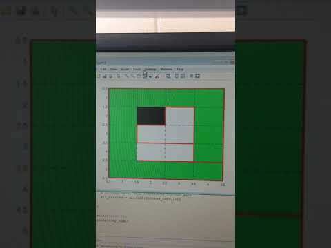
Note: We implemented a very baseline algorithm. You’ll see that the robot traverses the maze very inefficiently, especially when there are unvisitable areas; The robot has to return to its starting position to know if it has visited all unblocked grid spaces. There are many improvements you can make to this algorithm to make it as efficient as possible!

Real-time maze mapping

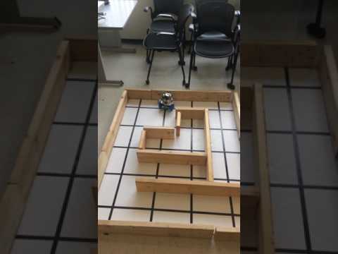
Once we were happy with our algorithm in simulation, we worked on implementing real-time navigation using that algorithm. We were able to use our line-following/turning code from Milestone 1. We also needed to be able to read the locations of front, left, and right walls at every intersection.
For wall detection, it was very important to translate the relative wall locations (front, left, right of the robot) into global wall locations (north, south, east, and west of the maze).
The navigation algorithm our robot uses to traverse the maze is the same as the algorithm in the Matlab simulation, with some additional support for getting wall information and for moving the robot.
Below is a video of the robot traversing a maze with the same wall configuration as in the simulation video above.

ECE 3400, Fall’17: Team Alpha

Milestone 3: Maze navigation algorithm

Matlab simulation

Real-time maze mapping