Cornell University: ECE 4960

Lab 11a: Turning a corner (Part I) - LQR on a Fast Robot

Objective

Lab 11a is the first of two labs that aim to make the robot perform full speed wall following along an interior corner. The objective of this first lab is to get a robot to do (straight-) wall following as fast as possible. This involves writing code infrastructure, approximating an A and a B matrix to describe the dynamics of your system, and implementing an LQR controller. Specifically, you will use feedback from your proximity sensor to keep your robot running at a specific distance from the wall while always keeping one motor at full speed. In the follow-on lab next week, we will improve this behavior using a Kalman Filter and make the robot perform a fast turn at an interior corner and continue wall following on the other side.

Parts Required

1 x Fully assembled robot, with Artemis, batteries, TOF sensor, and IMU.
An obstacle free path along a straight wall (min. 1.5m, preferably longer).
A white pillow or a sheet, or something to mitigate a potential crash.

Lab

Develop the lab infrastructure

Configure your robot, such that it has a tof sensor pointing forward, a proximity sensor pointing sideways (elevated over the wheels if possible to bring it closer to the wall), and an IMU.
Pay special attention to your proximity sensor – this is key to keeping you at a fixed distance from the wall.
- Find a good set-point value for the distance from the wall. Be sure to convert the proximity reading to [m].
- How fast can you read from the proximity sensor? What is the minimum and maximum distance at which you can rely on the data?
- Note that the sensor has a programmable integration time. If this is set too high, you will see large jumps in your data as the robot drives and you can no longer assume that the measurements are independent. You can lower the integration time (trading off accuracy for speed) using:
```
 proximitySensor.setProxIntegrationTime(4);   //1 to 8 is valid
```
Write software that lets you debug, record, and easily add functionality to the robot.
- You will need a function that updates all of the sensor values and system states. This function should be called in every loop.
- You will need a function that takes your computed input ‘u’, which can be positive and negative, and interprets it to motor commands between [0; 254].
```
 //Pseudocode:
 //Rescale u from torque (Nm) to motor values
 if(u <= 0)
 {
     uright = MAX_SPEED; //One motor should always run full speed
     uleft = MAX_SPEED+u;
 }
 else
 {
     uright = MAX_SPEED-u;
     uleft = MAX_SPEED; 
 }
```
- Each run is likely to take less than a second and things happen very fast, so you cannot debug these manually. Instead, we recommend creating one or more arrays to which you can append debugging messages that can be requested by and sent to the computer over Bluetooth after your run is over. You will likely have a lot of data to send, so it may be helpful to split it up over many packages. And remember the storage cannot exceed the RAM of 384kB.
- Since Lab 11-12a will consist of several pieces, we recommend using a Finite State Machine structure. Here is an example, but you are welcome to develop your own code. The cleaner this code is, the easier it will be for you to execute your lab. Remember to perform lots of unit checks to ensure that everything is working:
- Note that in this lab, we will only work with states 0-2. When state 2 is done, you can jump straight to state 5.
```
 // Pseudo code
 State 0: Setup. When setup is done, go to State 1.
 State 1: Ramp up to full speed open loop. After <RAMP_UP_TIME> go to
   State 2.
 State 2: Execute LQR control. When the ToF indicator sees a wall at
   <MIN_DISTANCE>, go to State 3.
 State 3: Execute a turn. When the robot measures a complete turn,
   go to State 4.
 State 4: Execute LQR control. After <MAX_TIME>, go to State 5.
 State 5: Stop the robot, and wait for a Bluetooth command requesting
   debugging data.  
```

Build your A and B matrix

To develop the LQR controller for wall following, we must first figure out how to describe our system in state space. Recall the A and B matrix discussed in Lecture 18. Since there are many things going on (drag, inter-motor forces, gear slack, etc.), we will make some simplifying approximations.
- For simplicity, we will assume that our only input is torque around the robot axis (driving it further or closer to the wall); and that the robot velocity is always close to the upper limit (i.e. the speed of the robot in m/s when both motors are set to 254). Our state space then includes [distance from the wall, d; the orientation of the robot, theta; the angular velocity of the robot, thetadot], where thetadot is included because the robot has momentum.
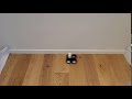
- First, recreate the situation you intend for your robot to work in, and study the system behavior as you apply a step response; i.e. drive your robot along a wall, after it has reached full speed, give it a step response. Choose parameters (i.e. a proximity and a step size) that is similar to what you expect from your final controller.
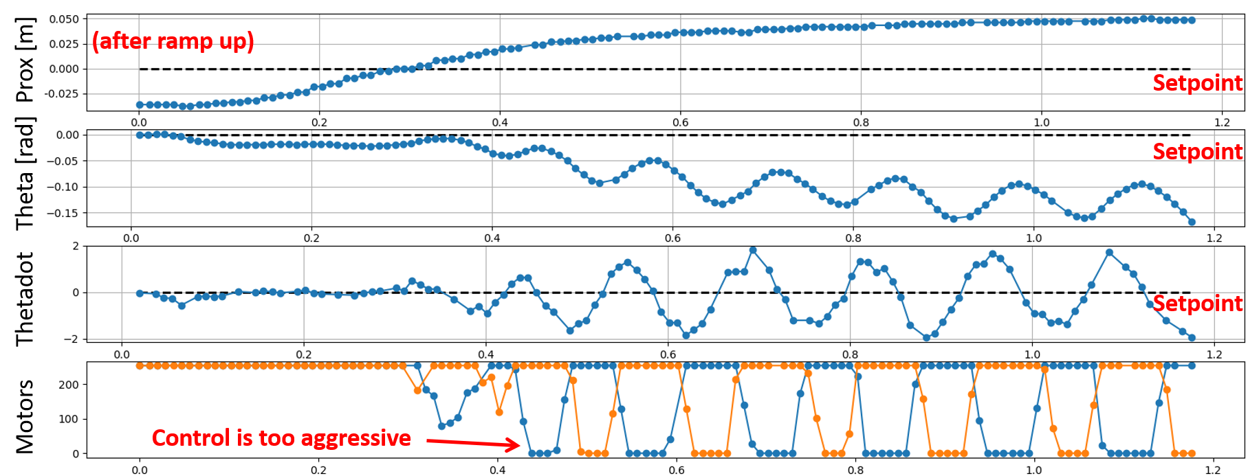
- Plot your data. You should find that the angular states behave like a second order system. We will capture this behavior in two variables related to momentum and damping/drag.
- Use the initial ramp up sequence, to find the maximum speed of your robot, v_max.
- Use the steady state response to estimate drag, d.
- Use the 90% rise time of to estimate inertia, I.
- Measure the approximate update rate (sampling time, Ts). You will use this in Lab 12a to work in discrete time.

LQR Wall following

Use the Python command listed below to compute a Kr matrix for wall following. Argue for your choice of Q and R. Note that you may have to experiment a bit with the real robot to get them right, depending on the behavior you see.

Remember, that our biggest concern is proximity to the wall, so you will need to penalize this state orders of magnitude more than theta and thetadot.

 Q = np.matrix([[..insert penalty1.., 0.0, 0.0, 0.0],
              [0.0, ..insert penalty2.., 0.0, 0.0],
              [0.0, 0.0, ..insert penalty3.., 0.0],
              [0.0, 0.0, 0.0, ..insert penalty4..]])
 R = np.matrix([..insert penalty5..])
 #solve algebraic Ricatti equation (ARE)
 S = scipy.linalg.solve_continuous_are(A, B, Q, R) 
 # Solve the ricatti equation and compute the LQR gain
 Kr = np.linalg.inv(R).dot(B.transpose().dot(S))   

Implement LQR control on your robot such that it can follow a wall at the distance you desire. You can use the BasicLinearAlgebra.h library to implement matrices.

 Matrix<1,2> Kr; 
 Matrix<1> u;
 Matrix<2,1> state;
 ...
 // Note that this format doesn't always work:
 Kr << value1, value2
 // But that this will:
 Kr(0,0)=value1;
 Kr(0,1)=value2;

Does the controller act as you expect it to given your cost functions?
- Try purposefully starting your robot at small proximity and angle offsets to help you answer this question.
- Look at your Kr-matrix. Given that we penalize proximity highest, why are the last two values not close to zero?
- How do you think a Kalman filter could help?

Write-up

To demonstrate that you’ve successfully completed the lab, please upload a brief lab report (<1.000 words), with code snippets (not included in the word count), photos, and/or videos documenting that everything worked and what you did to make it happen.