Cornell University: ECE 4960

Return to main page

Lab 12a: Turning a corner (Part II) - LQG on a Fast Robot

Objective

Lab 12a is the second of two labs that aim to make the robot perform high speed wall following along an interior corner. The objective of the second lab is to improve on (straight-) wall following by using a Kalman Filter to estimate the full state. An improved controller will allow the robot to hit the corner full speed and still manage to turn in time to engage with the second wall and continue wall following. Note that when you combine LQR with an optimal state estimator, we call this an LQG (linear quadratic gaussian) controller.

.

Parts Required

• 1 x Fully assembled robot, with Artemis, batteries, TOF sensor, and IMU.
• An obstacle free path along an interior corner (min. 1.5m x 1m, preferably longer).
• A white pillow or a sheet, or something to mitigate a potential crash.

Lab

Tune your Kalman Filter

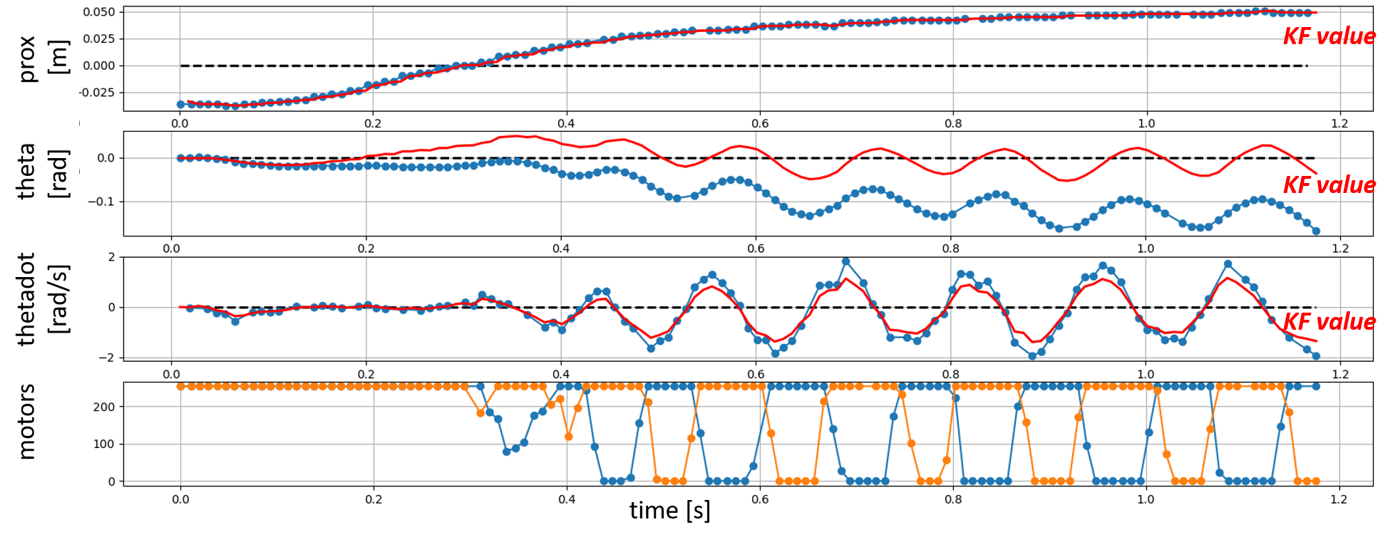
1. To improve the LQR wall following, we will develop a Kalman Filter that estimates the full state xhat = [proximity; theta; thetadot], given limited measurements y = [proximity; thetadot]. First, use the data you produced in Lab 11a to test how well your Kalman filter works before implementing it on the real robot. The following function is an example of how a Kalman Filter can be implemented in Python (refer to Lecture 18):
   • mu is the estimated state vector; sigma is the covariance matrix.
   • Subscripts “_ p” and “_ u” indicate the prediction and update step, respectively.
   • y_m is the difference between the measured (y) and predicted state (C * mu_p). E.g. if you measure proximity (state 1) and thetadot (state 3), C = [[1, 0, 0],[0, 0, 1]].
   • Sigma_u is the process noise covariance matrix, and Sigma_n is the measurement noise covariance matrix. Discuss your choice of Sigma_u and Sigma_n based on the real parameters of your robot, note that they may require tuning to get good performance.
   • Plot the KF estimated states on top the measured states to convince yourself (and us) that your estimator works as expected.

def kf(mu,sigma,u,y):
    
    mu_p = A.dot(mu) + B.dot(u) 
    sigma_p = A.dot(sigma.dot(A.transpose())) + Sigma_u
    
    y_m = y-C.dot(mu_p)
    sigma_m = C.dot(sigma_p.dot(C.transpose())) + Sigma_n
    kkf_gain = sigma_p.dot(C.transpose().dot(np.linalg.inv(sigma_m)))

    mu = mu_p + kkf_gain.dot(y_m)    
    sigma=(np.eye(3)-kkf_gain.dot(C)).dot(sigma_p)

    return mu,sigma

LQG Wall Following

1. Implement the code snippet above on your actual robot. As in Lab 11a, you can use the BasicLinearAlgebra.h library to initialize and perform matrix operations.
   • Since it can take a while for the Kalman Filter to regulate in on the actual robot state, it may be helpful to have this running during your ramp-up phase, even if there is no feedback control happening.
   • To convince yourself that everything is working as expected, consider adding both raw and estimated states to your debugging messages. If the robot doesn’t work at full speed, consider lowering your maximum speed a bit.

Turn the Corner

Next, instead of having the robot stop when it sees the wall, add on a 90 degree turn. Note that this turn must be fairly accurate for your robot to follow the second wall without crashing.

1. Get the timing just right! Your ToF sensor has a relative slow update rate. An update rate of, e.g. 0.1s, can lead to a forward displacement of 20cm at 2m/s, which will significantly affect your robot performance, as it exits the turn. You can in theory use the Kalman Filter to estimate the distance at a faster rate, but in this case it is easier to simply interpolate between your TOF measurements to produce a new estimated distance at the same rate as your other sensors. Your estimate will likely be inaccurate during your ramp-up phase because the robot is accelerating, but at maximum speed it should work well.

2. You can do the actual turn in several ways, the goal is to make the turning radius as small as possible.

   • You can try making it work open loop - this will be tricky, due to small deviations in the battery, the amount of slip, the angle with which the robot starts the turn, etc.
   • Check theta (integrated gyroscope Z reading) to see when you have reached 90 degrees.
   • If your robot turns too quickly after running at full speed, chances are that it is going to drift signficantly. If your drift is predictable, you can tune your controller to move your robot to the right position before re-engaging wall following. If the drift is not predictable, consider using PID control on the turning rate (similar to Lab 6), and lower the maximum rate of the turn such that the robot does not experience drift.
   • Feel free to come up with your own method.
   • Note that because the robot may continue to slide once you exit the turn, it may help to reengage both motors immediately after. For starters, you can simply set them both to full speed for a fixed time and worry about the LQR control later.

Re-engage LQR

1. For 3 extra credits, re-engage your LQR controller after the turn and demonstrate that you can turn reliably enough to make it work successfully. Remember to reset your setpoint for theta as the car will have turned 90 degrees.

Write-up

To demonstrate that you’ve successfully completed the lab, please upload a brief lab report (<1.000 words), with code snippets (not included in the word count), photos, and/or videos documenting that everything worked and what you did to make it happen.