Cornell University: ECE 4960
Lab 6(a): IMU, PID, and Odometry
Objective
The purpose of this lab is to setup your IMU (to enable your robot to estimate its orientation). Note that there are several ways to compute these, through this lab you should understand the trade offs of each approach. Once the IMU is implemented, you will mount it on your robot and attempt to do PID control on the rotational speed. Enabling reliable rotation will help you implement navigation and localization in labs 8-9; enabling reliable and slow rotation will help you do TOF rotational scans to compute a map in lab 7.
Parts Required
- 1 x SparkFun RedBoard Artemis Nano
- 1 x USB A-to-C cable
- 1 x Li-Ion 3.7V 400 or 500mAh battery
- 1 x Sparkfun Qwiic motor driver
- 1 x R/C stunt car and NiCad battery
- 1 x Qwiic connector
- 1 x 9-axis IMU
- 1 x TOF sensor
Prelab
- Consider installing SerialPlot to help visualize your data.
- Read up on the IMU Sparkfun documentation and datasheet.
- If you prefer to use the PID Arduino library instead of writing your own PID controller, you can find more information here
Lab Procedure
Set up your IMU
- Using the Arduino library manager, install the SparkFun 9DOF IMU Breakout - ICM 20948 - Arduino Library.
- Connect the IMU to the Artemis board using a QWIIC connector.
- Similar to the last lab, scan the I2C channel to find the sensor. Does the address match what you expected? If not, explain why.
- Run the “..\Arduino\libraries\SparkFun_ICM-20948\SparkFun_ICM-20948_ArduinoLibrary-master\examples\Arduino\Example1_Basics” and check out the change in sensor values as you rotate, flip, and accelerate the board. Explain what you see in both acceleration and gyroscope data.
Accelerometer
- Use the equations from class to convert accelerometer data into pitch and roll. To use atan2 and M_PI, you have to include the math.h library.
- Show the output at {-90, 0, 90} degrees pitch and roll. Hint: You can use the surface and edges of your table as guides to ensure 90 degree tilt/roll. If your table has soft corners, place your car on the floor and use the flat surfaces on it.
- How accurate is your accelerometer? You may want to do a two-point calibration (i.e. measure the output at either end of the range, and calculate the conversion factor such that the final output matches the expected output).
- Try tapping the sensor and plot the frequency response.
- At what frequencies is the unwanted noise? Here’s a helpful tutorial to do a Fourier Transform in Python
- Use these measurements to guide your choice of a complimentary low pass filter cut off frequency (recall implementation details from the lecture. Discuss how the choice of cut off frequency affects the output.
Gyroscope
- Use the equations from class to compute pitch, roll, and yaw angles from the gyroscope.
- Compare your output to the pitch and roll values from the accelerometer and the filtered response. Describe how they differ.
- Try adjusting the sampling frequency to see how it changes the accuracy of your estimated angles.
- Use a complimentary filter to compute an estimate of pitch and roll which is both accurate and stable. Demonstrate its working range and accuracy, and that it is not susceptible to drift or quick vibrations.
Magnetometer
- Use the equations from class to convert magnetometer data into a yaw angle.
<pre>
      xm = myICM.magX()*cos(pitch) - myICM.magY()*sin(roll)*sin(pitch) + myICM.magZ()*cos(roll)*sin(pitch); //these were saying theta=pitch and roll=phi
      ym = myICM.magY()*cos(roll) + myICM.magZ()*sin(roll_rad);
      yaw = atan2(ym, xm);
</pre>
- While keeping the IMU horizontal, change its orientation and find the magnetic north (feel free to ignore magnetic declination)
- Check that the output is robust to small changes in pitch
PID Control
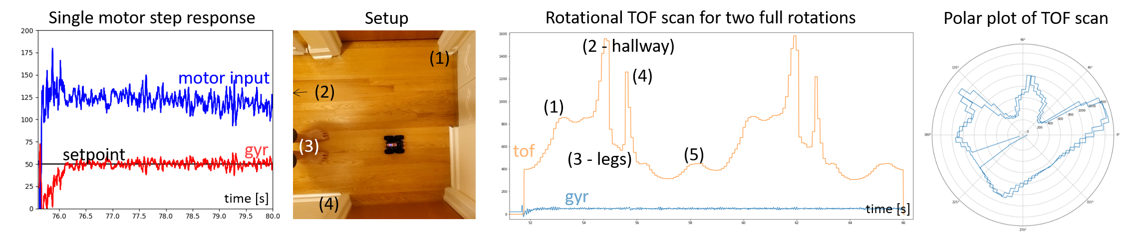
Recall, the objective of this lab is to make your robot rotate in a controlled manner. Controlled motion will help the robot localize and navigate during labs 8-9. If you can make it spin very slowly, this will help you take a rotational scan with your TOF sensor which will help you in lab 7 on mapping. Since one of the goals is to achieve slow and reliable rotation, it is highly unlikely to work on carpeted floors. If you don’t have access to hardwood or linoleum floors, consider taking your robot outside or even running it on a smooth table surface.
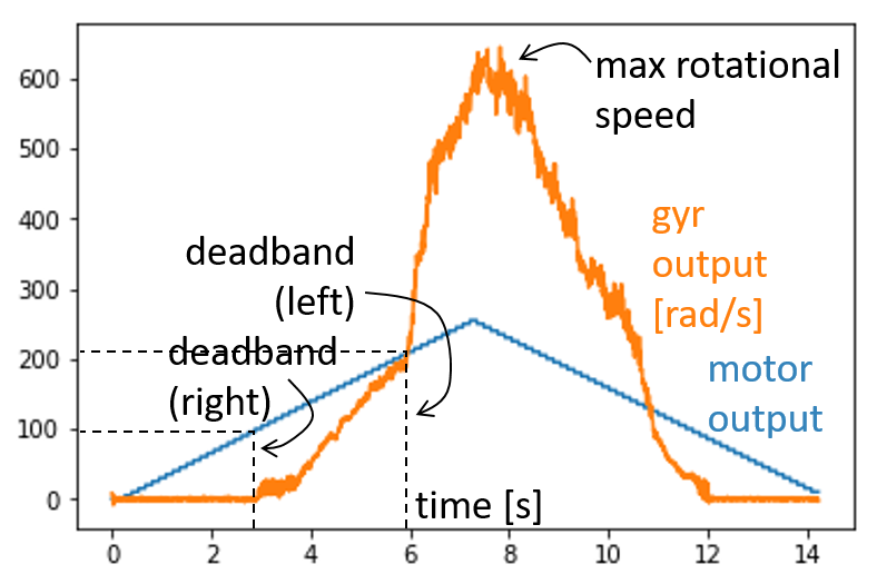
- Write a program to make the motors spin in opposite directions at increasing, followed by decreasing, speeds while recording yaw. In other words, create a ramp up and down function. Make sure that you change the motor values slowly, so that the robot can keep up with the changes. Execute your code with the robot sitting on a flat, smooth surface. Plotting your estimated yaw, what do you see? Examples may include:
- Maximum rotational speed
- Deadband (motor values below which the robot doesn’t spin)
- Hysteresis (the size of the deadband may depend on whether the motor value is increasing or decreasing).
- Differences between the motors (does one motor start/stop spinning before the other?)
-
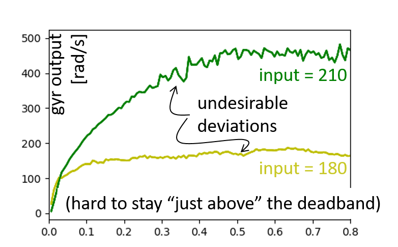
Guided by the ramp response, try finding the lowest possible speed at which you can reliably rotate your robot open loop around its own axis.
- Given the minimum speed of rotation that you found, reason about the accuracy of your TOF ranging.
- Determine the minimum sampling time of your TOF sensor (by measurement or datasheet).
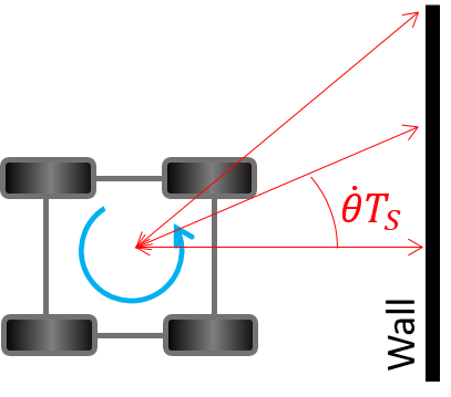
- If a robot starts, e.g. 0.5m from a wall pointing straight towards it, and spins as slowly as possible, how much does the orientation and distance change, before the measurement is done? If it starts angled 45 degrees to the wall, how much will it change now?
- Recall from lab 5 that the ToF sensor has two parameters, “signal and sigma”, that filters the output in case two consecutive measurements differ by too much. Reason about the feasibility of getting a reliable rotational scan given your system.
- Try implementing P, PI, or PID control (argue for your choice!) to make your robot rotate slowly around its own axis at a constant speed.
- Consider implementing wind-up protection if you incorporate an integral gain, and a low pass filter and derivative on the measurement if you implement a derivative gain.
- Describe your tuning method and results (feel free to use the heuristics or a step response and Cohen-Coon as mentioned in lectures).
- Note that when your setpoint is close to the deadband the non-linearity of your system is likely to cause trouble. First, choose a setpoint well into the linear range of your system, and use this setting to tune your gains and debug your code. Once that works, consider mapping (scaling and offsetting) the output from your PID controller to fit in the linear range of your system. Then try lowering your setpoint to make the robot spin as slowly as possible.
- What is the slowest you can make your robot reliably turn now? How does the behavior compare to open loop control? (I managed a stable speed of about half of what I could do open loop, can you beat my controller?)
- Most importantly, is this slow enough to produce a reliable rotational scan?

- You might very well need to make the robot spin almost an order of magnitude slower to produce reliable scans. One way to accomplish this is to give up spinning around the robot axis, and instead do feedback control on a single motor allowing the robot to spin in a wider circle. This will require some extra post processing in the mapping, localization, and navigation exercise, but it may very well be worth it. Alternatively, you can put effort into making the robot turn in small increments and only perform TOF ranging when the robot is stopped - given the hardware at your availability that might be very hard to get to work reliably. Since you already have PID control implemented at this point, let’s try the former!
- Apply PID control to one motor only and see how slow you can make the robot spin. What is the intuition for why you can achieve much lower speeds now?
- Note that if you set the motor controller for the passive side to 0, it will effectively break that motor, which may in turn cause your robot to drift additionally while spinning. To produce more reliable motion, consider applying a low value (e.g. 50) which will let the motor aid the other one just enough to allow the robot to spin around a single wheel.
- Given the lowest speed you were able to achieve, how much does the orientation of the robot change during a single measurement? If you were trying to map a 4x4m2 box and positioned in the middle, what kind of accuracy can you expect?
- If you’re eager, you can consider plotting the TOF sensor readings in a polar plot to try simple mapping. (Completely optional, as we will continue this excercise in the next lab)
- Optional : If you’re hooked on PID control by now (fun stuff, right??), consider implementing PID control on forward velocity using the TOF sensor as feedback (if it is pointing towards a wall, the decrement in distance will give you speed), or even directly on position with respect to the wall. Making this work now may ease navigation in lab 9. Be careful with overshoot, don’t let the robot hit the wall!
Write-up
To demonstrate that you’ve successfully completed the lab, please upload a brief lab report (<1.000 words), with code snippets (not included in the word count), photos, and/or videos documenting that everything worked and what you did to make it happen.
Lab 6(b): Odometry and Ground Truth in the Virtual Robot
Objective
The purpose of this lab is to learn to use the plotter tool and visualize the difference between the odometry and ground truth pose estimates of the virtual robot. This will provide you with a motivation for incorporating uncertainty into your robot model in future labs to effectively estimate and track its pose.
Prelab
**Odometry **
Odometry is the use of data from onboard sensors to estimate change in position over time. The relative changes recorded by the sensors (typically IMU and/or wheel encoders) are integrated over time to get a pose estimate of the robot. It is used in robotics by mobile robots to estimate their position relative to a starting location. This method is sensitive to errors due to the integration of velocity measurements over time to give position estimates.
The virtual robot provides simulated IMU data that mimics the one on the real robot, though the specific noise characteristics may differ. The simulated IMU data is integrated over time to give you the odometry pose estimate.
Ground truth
In robotics, ground truth is the most accurate measurement available. New methods, algorithms and sensors are often quantified by comparing them to a ground truth measurement. Ground truth can come either directly from a simulator, or from a much more accurate (and expensive) sensor.
In this lab, Ground truth is the exact position of your virtual robot within the simulator.
Virtual Robot
After completing Lab 5(b), you may have noticed that the virtual robot was fairly precise in its speed control. To save you time, the virtual robot does indeed come with a (simulated) constant speed controller and odometry pose estimation built in.
Plotter The 2d plotting tool is a lightweight process that allows for live asynchronous plotting of multiple scatter plots using Python. The Python API to plot points is described in the Jupyter notebook. It allows you to plot the odometry and ground truth poses. It also allows you to plot the map (as line segments) and robot belief in future labs. Play around with the various GUI buttons to familiarize yourself with the tool.
The plotter currently plots points only when the distance between subsequent points sent to it is greater than 0.03 m. This helps limit the number of points plotted. The value can be configured in the plotter config file plotter_config.ini present within the scripts folder.
Instructions
Workflow Tips
- Utilize the “Save the machine state” option when closing your VM. It is still recommended to restart your VM occasionally.
- To close the simulator gracefully, use the lab-manager terminal window. Refrain from quitting the simulator using other methods.
- You can close the lab-manager along with all the open tools by pressing <CTRL + C>.
Setup the base code
Download the lab6 base code and follow the setup instructions as per the previous labs.
Simulator and Plotter
- Start the lab6-manager:
lab6-manager- Notice there are now two tools available in the lab manager.
- Start the Simulator.
- Press <a> to select the simulator and <s> to start it.
- Start the Plotter.
- Press <b> to select the plotter and <s> to start it.
Keyboard teleoperation tool
To launch the keyboard teleoperation tool, open a new terminal and type in the command:
robot-keyboard-teleop
Jupyter Lab
- Start the Jupyter server in your VM from the work directory:
cd /home/artemis/catkin_ws/src/lab6/scripts- If the Jupyter server is stopped, you will not be able to run/open/modify any Jupyter notebooks.
- Open the notebook “lab6.ipynb” from the file browser pane in the left.
- Make sure the kernel is set to “Python 3”.
- This is shown in the top right corner of the notebook.
- The notebook should walk you through the exercise.
- SAVE your notebook after making changes, before closing the notebook or stopping the Jupyter server.
Tips
You may use the following questions to guide you through the lab exercise and write your report:
- How often do you send data to the plotter?
- Have you tested plotting large number of points and/or over long durations?
- Does the odometry trajectory look similar to that of the ground truth?
- What happens to the two plots when the robot is stationary?
- Does the noise in the odometry pose estimate differ with time/speed?
Write-up
To demonstrate that you’ve successfully completed the lab, please upload a brief lab report (<300 words), with code snippets (not included in the word count), photos, and videos documenting that everything worked and what you did to make it happen. Please add this write-up to the page you generated for Lab 6(a). You may use screen-recording tools from within the VM or on your host machine to record any necessary media.