Cornell University: ECE 4960 / 5960

Return to main page

Lab 7: Kalman Filter

Objective

The objective of Lab 7 is to implement a Kalman Filter, which will help you execute the behavior you did in Lab 6 fast, such that you can complete stunts in Lab 8. Remember to stick to the Task (A/B/C) you completed in Lab 6.

Parts Required

• 1 x Fully assembled robot, with Artemis, batteries, TOF sensor, and IMU.
• If you intend to do most of your testing at home, you’ll need to find an obstacle free path (at least 2m), and a bright pillow or similar to mitigate a potential crash. Remember, you will have to eventually re-calibrate everything to the lab floor where we will perform the stunts.

Lab Procedure

1. Step Response

Recall Lectures 11 and 12. To implement a Kalman Filter, you will need to estimate the terms in your A and B matrices using a step response.

• If you chose Task A or B, you will now use sensor fusion to help you estimate the distance to the wall frequently, inspite of the slow sampling time of the ToF sensor.
• If you chose Task C, you will now use sensor fusion to help you integrate ToF and gyroscope sensor values to estimate wall distance, orientation, and the rate of change in orientation.

Task A and B:

Execute a step response by driving the car towards a wall while logging motor input values and ToF sensor output.

1. Choose your step-size to be of similar size to the PWM value you used in Lab 6 (to keep the dynamics similar). If you never specified a PWM value directly, but rather computed one using your PID controller (Task A), pick something on the order of the maximum PWM value that was produced.
2. Make sure your step time is long enough to reach steady state (you likely have to use active breaking of the car to avoid crashing into the wall).
3. Show graphs for the TOF sensor output, the (computed) speed, and the motor input. Please ensure that the x-axis is in seconds.
4. Measure both the steady state speed and the 90% rise time and compute the A and B matrix.

Task C:

Execute a step response by driving the car straight at a constant speed, then slowing down one motor, while logging motor input values and gyroscope output.

1. Choose your initial motor value to be similar to the PWM value you used in Lab 6 (to keep the dynamics similar); and choose a step size (the decrease in PWM value to one motor) to be significant, such that you see clear results.
2. Make sure your car has achieved full speed before you apply your step, and make sure to execute the step long enough for the car to achieve constant angular speed.
3. Show graphs for the gyroscope sensor output, the (computed) orientation, and the motor input. Please ensure that the x-axis is in seconds.
4. Measure both the steady state angular speed and the 90% rise time, and compute the A and B matrix.

---

2. Kalman Filter Setup

1. For the Kalman Filter to work well, you will need to specify your process noise and sensor noise covariance matrices.
   • You will likely have to tune these according to what you see in the following step, but first try to reason about ballpark numbers for the variance of each state variable and sensor input here.
   • Recall that their relative values determines how much you trust your model versus your sensor measurements. If the values are set too small, the Kalman Filter will not work, if the values are too big, it will barely respond.
   • Recall that the covariance matrices take the approximate following form, depending on the dimension of your system state space and the sensor inputs.

sig_u=np.array([[sigma_1**2,0],[0,sigma_2**2]]) //We assume uncorrelated noise, therefore a diagonal matrix works.
sig_z=np.array([[sigma_4**2]])

1. Identify your C matrix. Recall that C is a m x n matrix, where n are the dimensions in your state space, and m are the number of states you actually measure.
   • For tasks A and B, this could look like: C=np.array([[-1,0]]), because you measure the negative distance from the wall (state 0).
   • For task C, this could look like: C=np.array([[1,0,0],[0,0,1]]), because you measure the distance from the wall (state 0) and the rate of change in angle (state 3).

---

3. Sanity Check Your Kalman Filter

Next, you will ensure that your Kalman Filter works by running it in Jupyter Lab on pre-recorded data from Lab 6.

1. Initialize your state vector, x.
   • For task A and B, this could look like: x = np.array([[-TOF[0]],[0]])
   • For task C, this could look like: x = np.array([[prox[0]],[theta[0]],[theta_dot[0]]])
2. Compute the discrete form of your dynamics matrix, A, and your input matrix, B. Since you will be running your Kalman Filter on old data, use the corresponding sampling time.

Ad = np.eye(n) + Delta_T * A  //n is the dimension of your state space 
Bd = Delta_t * B

1. Finally, implement your Kalman Filter using the function in the code below (for ease, variable names follow the convention from the lecture slides).
   • Prepare your data: For the function to work, you’ll need all input arrays to be of equal length. That means that you might have to interpolate data if for example you have fewer ToF measurements and motor input updates than you have recorded gyroscope data, due to the difference in sampling time. Numpy’s linspace and interp commands can help you accomplish this.
   • Loop through all of the data from your pre-recorded run, while calling this function. (If you are working on Task B, feel free to only include the first straight part of your run).
   • Remember to scale your input from 1 to the actual value of your step size (u/step_size).
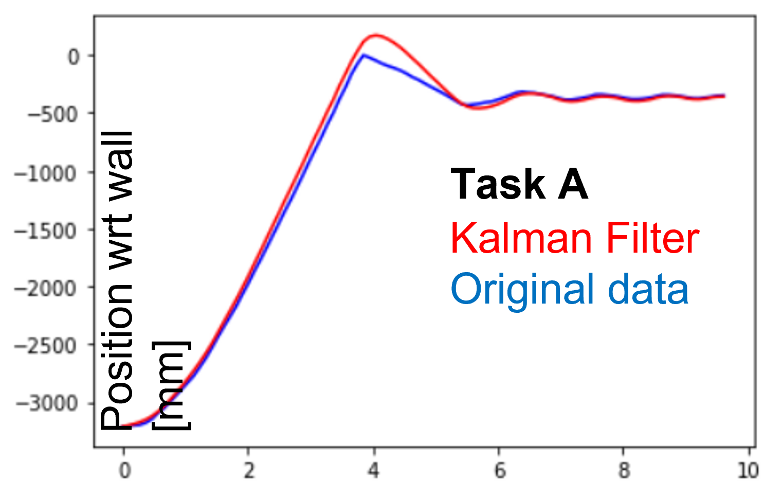
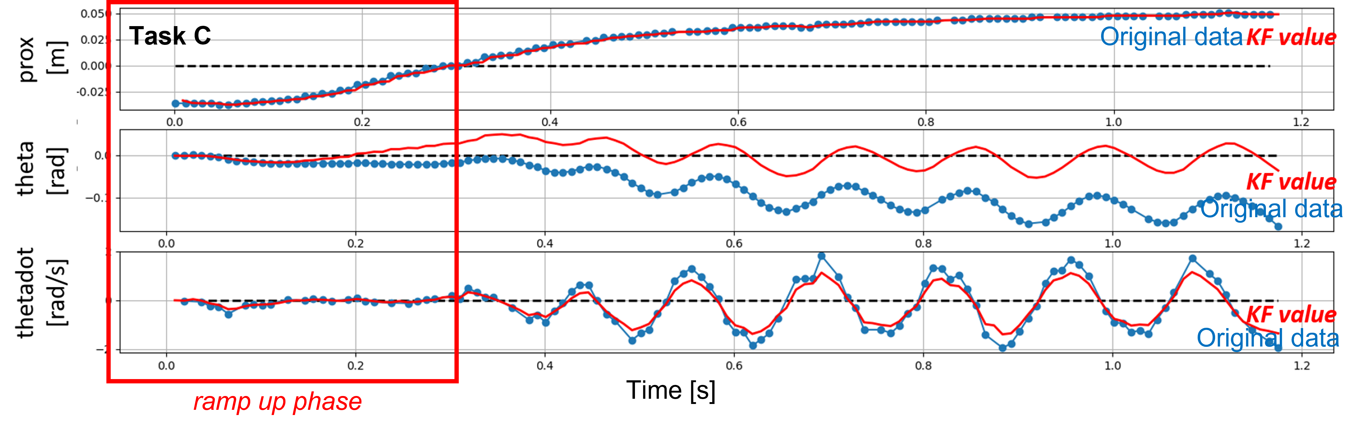
   • Plot the Kalman Filter output to demonstrate how well your Kalman Filter estimates your system state.
   • If your Kalman Filter is off, try adjusting your covariance matrices. Discuss how/why you adjust them.

def kf(mu,sigma,u,y):
    
    mu_p = A.dot(mu) + B.dot(u) 
    sigma_p = A.dot(sigma.dot(A.transpose())) + Sigma_u
    
    sigma_m = C.dot(sigma_p.dot(C.transpose())) + Sigma_z
    kkf_gain = sigma_p.dot(C.transpose().dot(np.linalg.inv(sigma_m)))

    y_m = y-C.dot(mu_p)
    mu = mu_p + kkf_gain.dot(y_m)    
    sigma=(np.eye(3)-kkf_gain.dot(C)).dot(sigma_p)

    return mu,sigma

4. Implement the Kalman Filter on the Robot

Finally, integrate the Kalman Filter into your Lab 6 PID solution on the Artemis. While you don’t have to try to increase this speed of your current solution, you should compute the Kalman Filter locally on your robot, and verify via your debugging script that it works as expected.

The following code snippets gives helpful hints on how to do matrix operations on the robot:

#include <BasicLinearAlgebra.h>  //Use this library to work with matrices:
using namespace BLA;             //This allows you to declare a matrix

Matrix<3,1> state = {0,0,0};     //Declares and initializes a 3x1 matrix 
Matrix<1> u;                     //Basically a float that plays nice with the matrix operators
Matrix<3,3> A = {1, 1, 0,
                 0, 1, 1,
                 0, 0, 1};       //Declares and initializes a 3x3 matrix
state(1,0) = 1;                  //Writes only location 1 in the 3x1 matrix.
Sigma_p = Ad*Sigma*~Ad + Sigma_u; //Example of how to compute Sigma_p (~Ad equals Ad transposed) 

Write-up

To demonstrate that you’ve successfully completed the lab, please upload a brief lab report (<800 words), with code snippets (not included in the word count), photos, and/or videos documenting that everything worked and what you did to make it happen.