Cornell University: ECE 4960
Lab 7(a): Grid Localization using Bayes Filter
Objective
The lab serves as a precursor to the next lab where you will be implementing grid localization using Bayes Filter. Implementation in robotics can be a daunting task with multiple sub-objectives. It is always a good idea to list out the sub-objectives for your task and modularize your code accordingly. The Jupyter notebook provides you with a skeleton code and some helper functions to get the job done. Read through the documentation and write pseudo code for the localization functions in the notebook. You are not required to write any python code to implement the Bayes filter. Try to be very concicse - this will improve our feedback comments and ease the actual implementation in the next lab.
Background
Robot Localization
Robot localization is the process of determining where a mobile robot is located with respect to its environment. Plotting odometry against the ground truth in the previous lab should have convinced you that non-probabilistic methods lead to poor results.
Odometry
Odometry is the use of data from onboard sensors to estimate change in position over time. The virtual robot provides simulated IMU data that mimics the one on the real robot, though the specific noise characteristics may differ. The simulated IMU data is integrated over time to give you the odometry pose estimate.
Ground truth
In robotics, Ground truth is the most accurate measurement available. New methods, algorithms and sensors are often quantified by comparing them to a ground truth measurement. In this lab, ground truth is the exact pose of your virtual robot in the simulator.
Grid Localization
The robot state is 3 dimensional and is given by . The robot’s world is a continuous space that spans from (-2,+2)m in the x direction, (-2,+2)m in the y direction and [-180,+180) degrees along the theta axis. There are infinitely many poses the robot can be at within this bounded space.
We discretize the continuous state space into a finite 3D grid space, where the three axes represent ,
and
. This reduces the accuracy of the estimated state as we cannot distinguish between robot states within the same grid cell, but allows us to compute the belief over a finite set of states in reasonable time.
The grid cells are identical in size. The size of each grid cell (i.e resolution of the grid) along the ,
and
axes are 0.2m, 0.2m and 20 degrees, respectively. The number of cells along each axis is (20,20,18). Each grid cell stores the probability of the robot’s presence at that cell. The belief of the robot is therefore represented by the set of probabilities of each grid cell and these probabilities should sum to 1. The Bayes filter algorithm updates the probability of the robot’s presence in each grid cell as it progresses. The grid cell(s) with the highest probability (after each iteration of the bayes filter) represents the most probable pose of the robot. Thus the most probable cell across different time steps characterizes the robot’s trajectory.

The robot is initialized with a point mass distribution at (0,0,0) which translates to the grid cell index (10,10,9). This can be calculated using the grid resolution, grid size, and the fact that indices start from 0. The initial probability at the grid cell index (10,10,9) is 1 and every other cell has a value of 0.
The image above depicts the 3d grid model. The green cell depicts the grid cell index (10,10,9). The top, middle and bottom x-y grid planes depict all the discrete robot states where the third index is 0, 9 and 17, respectively.
Sensor Model
We utilize a Gaussian Distribution to model the measurement noise. This can be thought of as a simplified version of the Beam model where we ignore the remaining three distributions used to model failures, unexpected objects, and random measurements. This simplified model works surprisingly well for laser range finders operating in static, indoor environments. Refer lecture 10.
Motion Model
You should utilize the odometry motion model for this lab. At every time step, we can record the odometry data before and after the movement. This relative odometry information can be described by the motion parameters: rotation1, translation and rotation2. Refer lecture 11. You can use the Gaussian Distribution to model the noisy control data in the odometry motion model.
Bayes Filter Algorithm
Essentially, every iteration of the Bayes filter has two steps:
- A prediction step to incorporate the control input (movement) data
- An update step to incorporate the observation (measurement) data
The prediction step increases uncertainty in the belief while the update step reduces uncertainty. The belief calculated after the prediction step is often referred to as prior belief. Refer lecture 8 and lecture 9.
Instructions
Workflow Tips
- To close the simulator gracefully, use the lab-manager terminal window. Refrain from quitting the simulator using other methods.
- You can close the lab-manager along with all the open tools by pressing <CTRL + C>.
- You can double click left of a cell in a Jupyter notebook to collapse it to a single line. Double clicking again will expand the cell.
- If the plotter becomes sluggish over long operating times, restart it.
- There is a small “A” button on the bottom left corner of the plotter tool that zooms the plot to fit in the window.
Setup the base code
Download the lab7 base code and follow the setup instructions as per the previous labs.
Simulator and Plotter
Use the lab7-manager to start the simulator and the plotter.
Jupyter Lab
- Start the Jupyter server in your VM from the work directory:
cd /home/artemis/catkin_ws/src/lab7/scripts- If the Jupyter server is stopped, you will not be able to run/open/modify any Jupyter notebooks.
- Open the notebook “lab7a.ipynb” from the left file browser pane.
- Make sure the kernel is set to “Python 3”. This is shown in the top right corner of the notebook.
- The notebook should walk you through the exercise.
- Hint: In the prediction step of the Bayes filter, you will need to cycle through all possible previous and all possible current states in the grid to estimate the prior belief (bel_bar). Think about how many loops would be required to perform this.
- SAVE your notebook after making changes, before closing the notebook or stopping the Jupyter server.
Write-up
To demonstrate that you’ve successfully completed the lab, please upload a brief lab report (<600 words), with concise pseudo code (not included in the word count), photos, and videos documenting that everything worked and what you did to make it happen. You may use screen-recording tools from within the VM or on your host machine to record any necessary media.
Lab 7(b): Mapping
Objective
The purpose of this lab is to build up a map of your room (or another static environment you have access to). The quality of these maps will rely on how well you managed to perform PID control on turning in the last lab. Remember, when robots in the real world rely on maps, they also have to deal with inconsistencies that arise from the limited quality of their own controllers. However, if you had a lot of trouble getting lab 6 to work, you can also manually calibrate your map using a tape measurer - if you do so, please note it on your write-up!
To limit the processing time of the simulator and localization algorithm, we request that you map out a space that is no more than 4m x 4m.
Parts Required
- 1 x Fully assembled robot, with Artemis, batteries, TOF sensor, and IMU. A tape measure will also be very helpful!
Prelab
- Consider checking out lecture 2 on transformation matrices again.
Lab Procedure
Use the robot to generate a map
- Prepare the room to be mapped out.
- The room needs to be static (so that you can use this map for the next two weeks). If you need to move things, use the tape to mark where things were so that you can recreate the setup whenever you want to. You are welcome to add tape to the floor of PH427 as well, but please move it when this lab sequence is over.
- The floor needs to match what you got your PID controller working on. If your room has carpets, consider running your robot in a bathroom/kitchen or even outside. If you are on campus, you can use PH427, but please setup your own scenario so that not everyone has the same map.
- The TOF sensor will work best with big even surfaces, such as walls, boxes, and bed spreads that reach the floor without too many folds. In other words, this lab will be easier if you remove ground clutter from the floor. Eventually we will incorporate this map into the discrete occupancy grid in the simulator with 0.2m x 0.2m cells, so features smaller than this may not come out well.
- Make it interesting! Please add at least one “island” (or a peninsula) in the middle of the open space which the robot can navigate around in the next lab. The island can be a bed pressed up against a wall or simply one or more boxes in the middle of the room.
- Break the symmetry. Think about how the robot will estimate its localition given a rotational scan. If your map is completely symmetrical, the robot will have a hard time estimating where it is. Use the “island” or other landscape features to break the symmetry to allow the robot to quickly narrow down its location.
- Sanity check!
- Make your robot do a single rotation near a corner of the room while measuring the distance with the TOF sensor and the orientation with the gyroscope.
- Try plotting the output as a polar coordinate plot. For simplicity assume that the robot rotated in place. Do the measurements match up with what you expect?
- To ease debugging, we strongly recommend grabbing all the raw data measured by the robot and sending it over Bluetooth to your computer for postprocessing.
- Avoid unnecessary delays in your control loop. E.g make sure that you don’t wait for the TOF sensor data to be ready. Similarly, consider saving all the data in arrays and sending them over Bluetooth after your robot is done with the scan.
- Try rotating twice and see how reliable the scan is. The reliability will depend on the accuracy of your PID controller. If you had trouble getting the PID to work, consider turning the robot in small increments instead and perform your measurements while the robot is sitting still.
- Explain what you see and any sources of inconsistency in terms of angle increments and/or range measurements.
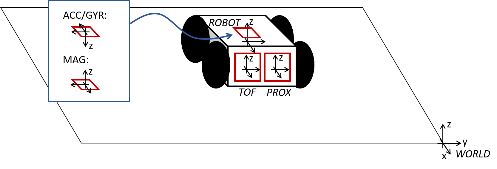
- Compute the transformation matrices and convert the measurements from the distance sensor to the inertial reference frame of the room. These will depend on how you mounted your sensors on the robot.
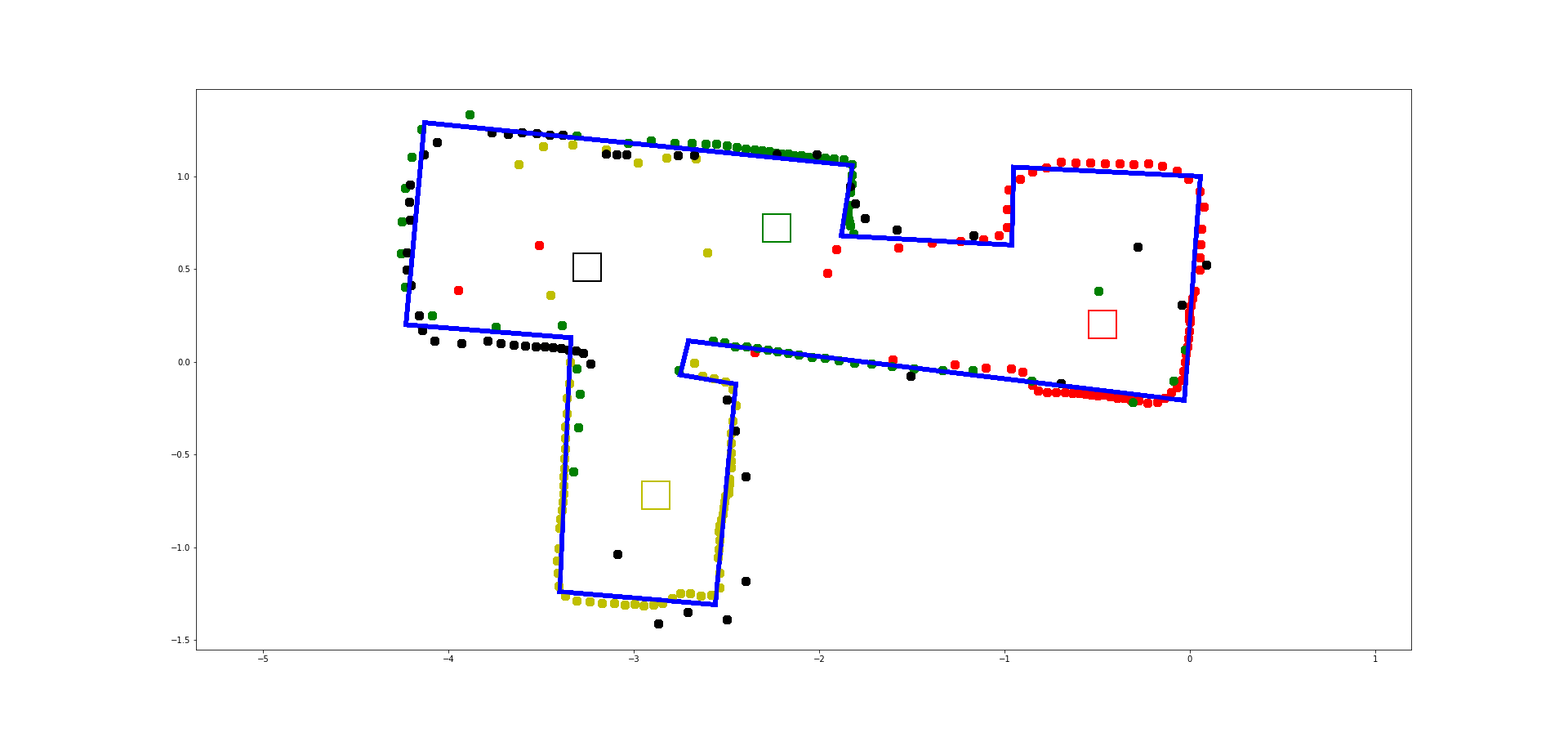
- Build your map by manually placing your robot in known poses with respect to the inertial frame, and perform line scans. The number of scans you need will depend on the complexity of the room you are trying to map out. Collect data from all of your line scans to make a scatter plot that resembles a map of your room. Remember to keep within a 4m x 4m space.
- To make it easier on yourself, start the robot in the same orientation in all scans.
- If you don’t have a tape measure to measure the pose, use the robot and the TOF sensor itself. Point it straight towards a wall while sitting still, take the average of several measurements and let that give you an estimate of x and y in the inertial frame.
- Please add a sketch showing what the room actually looks like, so we can help you debug if things don’t look right.
- To convert this into a format we can use in the simulator, manually guess where the actual walls/obstacles are based on your scatter plot. Draw lines on top of these, and save two lists of the end points of these lines: (x_start, y_start) and (x_end, y_end).
- Note that if the number of tof measurements varies between rotations, you may have to pair your readings down to a fixed number (you read earlier that the simulator expects scans in 20 degree increments corresponding to 18 readings at equal intervals around a 360 scan). Argue for how you pair down your readings (avg? sample based? interpolation? etc.).
Visualize your map in the Plotter tool
The map will be used in future labs and so it is a good idea to know if it looks as expected in the plotter tool as well.
Open the notebook “lab7b.ipynb” in your VM and follow the instructions.
Write-up
To demonstrate that you’ve successfully completed the lab, please upload a brief lab report (<8.00 words), with code snippets (not included in the word count), photos, and/or videos documenting that everything worked and what you did to make it happen. Please add this write-up to the page you generated for Lab 7(a).